An Introduction to Manifold

Content

• Exterior Algebra of Multicovectors

  • Tensor Product

  • Wedge Product

• Linearization of Manifold

  • Tangent Space

  • Tangent Bundle

  • Differential Form

• Linearization of Mapping

  • Differential of Mappings (Pushforward)

  • Pullback

• Calculus on Manifold

  • Exterior Derivative

  • Integration

• Miscellaneous

Exterior Algebra of Multicovectors

Motivation

Instead of working with tangent vectors, it turns out to be more fruitful to adopt the dual point of view and work with linear functions on a tangent space. After all, there is only so much that one can do with tangent vector, which are essentially arrows, but functions, far more flexible, can be added, multiplied, scalar-multiplied and composed with other maps.

Tensor Product

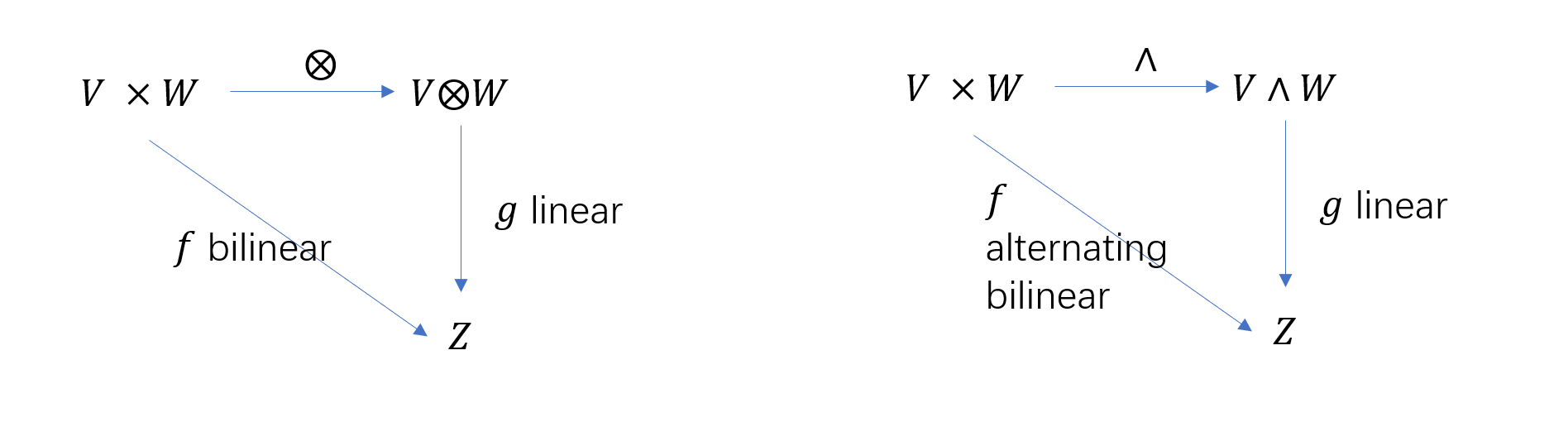
One of the motivations to define tensor product is to convert a bilinear mapping over $V \times W$ into a linear mapping, i.e., given $f: V\times W \rightarrow Z$, find vector space $Y$ and bilinear mapping $h:V\times W \rightarrow Y$ such that there exists a unique linear mapping $g: Y\rightarrow Z$ satisfying $f = g\circ h$. The space $Y$ is exactly the tensor product of $V$ and $W$. (A commutative diagram is helpful to understand the relation.)

Denote the space of all $k$-linear function $f: V_1 \times \cdots \times V_k \rightarrow \mathbb{F}$ as $\mathscr{L}(V_1, \cdots, V_k; \mathbb{F})$, $V^*$ is dual space of $V$.

Firstly, define the tensor product operation between linear functions

Secondly, define the tensor product between vector spaces

One can verify that

• $V^\ast \otimes W^\ast = \mathscr{L}(V, W; \mathbb{F})$, $V\otimes W :=\mathscr{L}(V^{\ast} , W^{\ast} ; \mathbb{F})$
• $(a^{\ast i} \otimes b^{\ast \alpha})$ is a basis for $V^{\ast} \otimes W^{\ast} $ where ${a^{\ast i}, 1\leq i\leq n}$ is a basis of $V^{\ast} $, ${b^{\ast \alpha}, 1\leq \alpha\leq m}$ is a basis of $W^{\ast} $.
• $\mathscr{L}(V, W; Z)$ is isomorphic to $\mathscr{L}(V\otimes W; Z)$ where $Z$ is another vector space over $\mathbb{F}$.

The properties above show that the tensor product achieve our target and it can be generalized to multilinear function easily.

DEF: Let $f$ be a $k$-linear function and $g$ an $l$-linear function on a vector space $V$. Their tensor product is the $(k+l)$-linear function $f\otimes g$ defined by

DEF: Suppose $V$ is a $n$-dimensional vector space and its dual space is $V^*$, then we call the element of tensor product

as $(r, s)$-type tensor, which should be treated as a multillinear function instead of a vector. In practice, we always abuse this word in different scenarios, especially when we are talking about the “tensor product” of vectors.

NOTE: The definition above is rather abstract but still gives a way of putting vector space together to form larger vector spaces, which is crucial to the quantum mechanics of multi-particle systems. And from this view point we can further derive the frequently-used Kronecker product of matrices.

Now we have constructed a new form of vector spaces, what sorts of linear operators act on the space $V \otimes W$?

Suppose $v$ and $w$ are vectors in $V$ and $W$, and $A$ and $B$ are linear operators on $V$ and $W$, respectively. Then we can define a linear operator $A \otimes B$ on $V \otimes W$ by

Consider its matrix representation, we index a basis for $V\otimes W$ as $u_{k} = v_i \otimes w_j$ for $i=1, \cdots, n$, $j=1, \cdots, m$ and $k= (i-1)n + j$. Thus, $A \otimes B$ is a $mn$-by-$mn$ matrix and

furthermore,

Remark:

From the prospect of constructing larger vector spaces from small vector spaces according to some commutative diagram, we have the following comparison between tensor product and wedge product.

Wedge Product

DEF: For alternating multilinear function $f\in A_k(V)$ and $g\in A_l(V)$, where $A_k(V)$ denoting the space of all alternating $k$-linear functions on a vector space $V$ for $k>0$, we would like to have a product that is alternating as well, then we define their wedge product (exterior product) as

where $S_k$ is the group of all permutations of the set ${1, \cdots, k}$.

Properties of wedge product

• Anti-commutative : $f \wedge g = (-1)^{k+l} g \wedge f$, $f\in A_k(V), g\in A_l(V)$.
• Associativity : $(f \wedge g) \wedge h = f \wedge (g \wedge h)$.

In general, one can verify that

If $\alpha^1, \cdots, \alpha^k$ are linear functions on a vector space $V$ and $v_1, \cdots, v_k\in V$, then

Furthermore, all the alternating $k$-linear function $\alpha^I$ with $I=(i_1 < \cdots < i_k)$ form a basis for the space $A_k(V)$.

Note: For a vector in $A_k(V)$, it can be written as $\xi=\xi_{i_1\cdots i_r} e_{i_1} \otimes \cdots \otimes e_{i_r}$ or

there is a scalar difference between inner products for $e_{i_1} \otimes \cdots \otimes e_{i_r}$ and $e_{i_1} \wedge \cdots \wedge e_{i_r}$.

Linearization of Manifold

Tangent Space

There are several equivalent definitions for tangent, each gives the convenience to address some specific questions.

• In the view of abstract operation rule

  A tangent vector at a point $p$ is a linear map $D:C^{\infty}_p \rightarrow \mathbb{R}$ such that $D(fg)=D(f)g + fD(g)$.

• In the view of velocity vector of curves

  A tangent vector $X_p$ at a point $p$ of a manifold $M$ associated with a smooth curve $c:(-\varepsilon, \varepsilon)\rightarrow M$ starting at $p$ with $c(0)=p$, is a map $X_p:C^{\infty}_p \rightarrow \mathbb{R}$ such that for any $f\in C^{\infty}_p$,

  \[X_p f = \left.\frac{\mathrm{d}}{\mathrm{d}t} \right\vert_{t=0} (f \circ c), \quad X_p=c'(0).\]

Note: some discussion for the equivalent class in the definition above is necessary but we omit here. Actually, the first gives the direct definition of tangent space while the second one treat it as the dual space of cotangent space.

Tangent Bundle

A smooth vector bundle over a smooth manifold $M$ is a smoothly varying family of vector spaces, parametrized by $M$, that locally looks like a product.

A $C^{\infty}$ vector bundle of rank $r$ is a triple $(E, M, \pi)$ consisting of manifolds $M$ and $E$, and a surjective smooth map $\pi:E\rightarrow M$ that is locally trivial of rank $r$. The manifold $E$ is called the total space of the vector bundle and $M$ the base space.

The tangent bundle of a manifold $M$ is a triple $(TM, M, \pi)$.

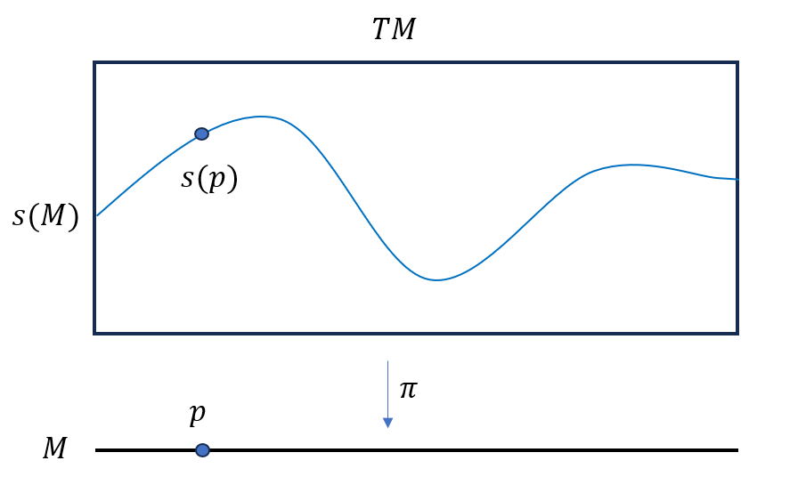
A section of a vector bundle $\pi: E\rightarrow M$ is a map $s: M \rightarrow E$ such that $\pi \circ s=1_{M}$, i.e., for each point $p$ in $M$, $s$ maps $p$ into the fiber $E_p$ above $p$. Visualization see the figure below, which somehow shows why we define the vector bundle and its section.

NOTE: $C^{\infty}$ section can be operated like trivial function, and the set of all $C^{\infty}$ sections of $E$ is denoted by $\Gamma(E)$, which is not only a vector space over $\mathbb{R}$ but also a module over the ring $C^{\infty}(M)$ of $C^{\infty}$ functions on $M$.

Vector fields, which manifest themselves in the physical world as velocity, force, electricity, magnetism, and so on, may be viewed as sections of the tangent bundle over a manifold.

Differential Forms

Differential forms are generalization of real-valued functions on a manifold. Instead of assigning to each point of the manifold a number, a differential $k$-form assigns to each point a $k$-covector on its tangent space.

For $k=0$ and $k=1$, differential forms are functions and covector fields respectively.

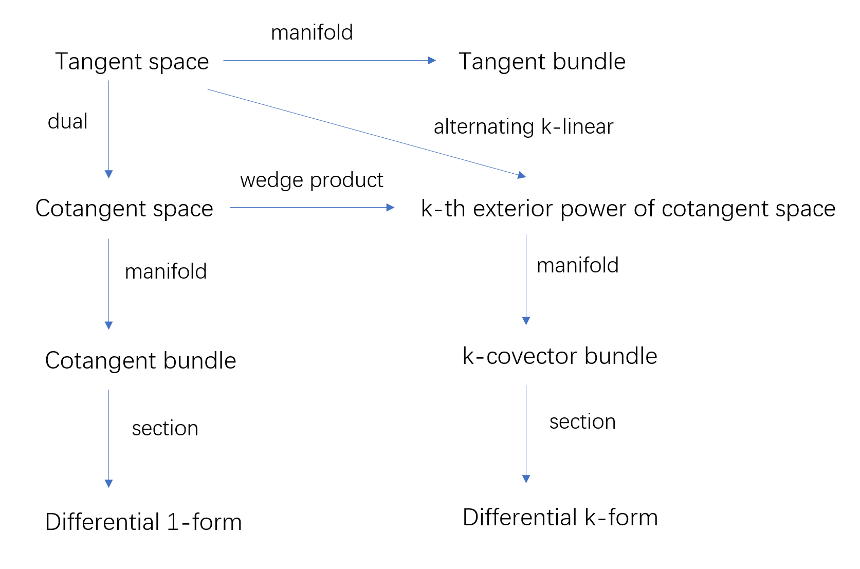
Specifically, we have the following graph stating the relations between tangent space, tangent bundle, cotanget space, cotangent bundle, $k$-covector bundle and differential $k$-form. They all can be treated as the special linear structure arising over the manifold.

Differential $1$-form over $\mathbb{R}^n$

A differential 1-form, or a covector field on smooth manifold $M$, is a function $\omega$ that assigns to each point in $M$ a covector $\omega_p$ at $p$.

If $f$ is a $C^{\infty}$ real-valued function on manifold $M$, its 1-form $\mathrm{d}f: T_pM \rightarrow \mathbb{R}$ such that for any $p\in M$ and $X_p\in T_p M$,

Remark:

Motivated by the calculation for velocity vector,

there are two elements $f, \gamma$, which can be treated as a bilinear pair. However, there are not linear and one-by-one, we have to introduce the equivalent class for this two elements and lead to the concepts of vector field (tangent vector) and differential of functions (1-form).

Consider the bilinear pairing:

One may think of a tangent vector as a function on the second argument of this pairing $X_p = \langle X_p, \cdot \rangle$. And the differential $(df)_p$ at $p$ is a function on the first argument of the pairing $(df)_p = \langle \cdot, f \rangle$. To create an inner product pair, we should take the dual pair $T_p$ and $T^*_p$ and denote

Only in this sense we have the linear property for each component. For example

Be careful with notation here.

Differential $k$-form over $\mathbb{R}^n$

Just as a vector field assigns a tangent vector to each point of an open subset $U$ of $\mathbb{R}^n$, dually a differential $k$-form assigns a $k$-covector on the tangent space to each point of $U$.

DEF: A differential form $\omega$ of degree $k$ on an open subset of $\mathbb{R}^n$ is a function $\omega(p) := \omega_p \in A_k(T_p(\mathbb{R}^n))$, such that

where $1 \leq i_1 < \cdots < i_k \leq n $.

Linearization of Mappings

A basic principle in manifold theory is the linearization principle, according to which a manifold can be approximated near a point by its tangent space at the point, and a smooth mapping can be approximated by the differential of the map. In this way, one turns a topological problem into a linear problem.

Further Examples

• Inversion function theorem: invertibility of smooth map –> invertibility of its differential at a point

• Regular level set theorem: a level set all of whose points are regular is a regular submanifold, i.e., a subset that locally looks like a coordinate $k$-plane in $\mathbb{R}^n$.

Given two manifolds, there are several ways to linearize the mapping between these two manifolds due to the different “linearization structures of a manifold”.

Differential of Mappings (Push forward)

Let $F: N\rightarrow M$ be a $C^{\infty}$ map between two manifolds. At each point $p\in N$, the map $F$ induces a linear map of tangent spaces, called its differential at p, $F_* : T_p N \rightarrow T_{F(p)} M$, defined as

Similar to the equivalent definition of tangent vector, we can also compute the differential of the smooth mapping utilizing the smooth curve, i.e.,

where $c$ is a smooth curve starting at $p$ with velocity $X_p$ at $p$, i.e., $c(0)=p, c’(0)=X_p$.

NOTE: we call it differential of the mapping for the reason that it connects two tangent spaces and possess the chain rule:

Remark: Differential of mappings (denoted by $F_*$) are different with differential of functions (or differential 1-form, denoted by $\mathrm{d}f$). The first one is considering about the structure between two manifolds, while the last one is talking about the structure over single manifold.

Pullback

Pullback of functions

Let $F: M\rightarrow N$ be a map and $h$ a function on $M$. Then pullback of $h$ by $F$, denoted as $F^*h$, is the composite function $h\circ F$.

Pullback of differential 1-form

Suppose $F:M\rightarrow N$ is a smooth mapping, $p\in M, q=F(p)$. Then one can induce the linear mapping between the cotangent spaces $F^* : T_q^* \rightarrow T_p^* $:

NOTE: we call it pullback for the reason that after compositing with $F$, both $u\circ F$ and $v\circ F$ are function in $C^{\infty}(M)$ instead of $C^{\infty}(N)$.

Pullback of differential k-form

Finally, we can generalize the linear mapping from cotangent space $T_q^*$ to exterior algebra space $A(N)$,

For $\beta\in A^r(N)$($r\geq 1$), define

For $\beta\in A^0(N)$, define

Calculus on Manifold

Exterior Derivative

In contrast to undergraduate calculus, where the basic object of study are function, the basic objects in calculus on manifolds are differential forms. Now we show how to differentiate differential forms.

Here is the first time we introduce the word “exterior” seriously.

Exterior derivative over $\mathbb{R}^n$

Denote by $\Omega^k(U)$ the vector space of $C^{\infty}$ $k$-forms on $U$.

To define the exterior derivative of a $C^{\infty}$ $k$-form on an open subset $U \subset \mathbb{R}^n$, we first define it on $0$-forms:

• For $f\in C^{\infty}(U)$, the exterior derivative is defined as it differential $\mathrm{d}f \in \Omega^1(U)$, in terms of coordinate

• For $k\geq 1$, if $\omega=\sum_I a_I \mathrm{d}x^I \in \Omega^k(U)$, then

Properties of Exterior Derivative

• $\mathrm{d}(\omega \wedge \tau) = (\mathrm{d}\omega) \wedge \tau + (-1)^{\mathrm{deg}(\omega)}\omega \wedge \mathrm{d}\tau$. ($-1$ comes from the anti-commutative of wedge product)
• $\mathrm{d}^2 = 0$
• If $f\in C^{\infty}(U)$ and $X$ be $C^{\infty}$ vector field, then $(\mathrm{d}f)(X) = Xf$.

Remark: The properties above uniquely characterize exterior differentiation on $U$, which can be regarded as another definition of exterior derivative.

NOTE: We use the same notation $\mathrm{d}$ for exterior derivative and differential of function. But differential of function are only a special case of exterior derivative. The word “Exterior’’ appeared here mainly afford the alternating-linear property of $k$-forms.

Integration

Orientations

For integration over a manifold to be well defined, the manifold needs to be oriented.

Orientation of a vector space

An orientation of a finite-dimensional real vector space is an equivalence class of ordered bases: two ordered bases being equivalent if and only if their transition matrix has positive determinant.

Instead of using an order basis, we can also use an $n$-covector to specify an orientation based on the fact that the space of $n$-covectors is one-dimensional. Further, we say that the $n$-covector $\beta$ specifies the orientation $(v_1, \cdots, v_n)$ if $\beta(v_1, \cdots, v_n) > 0$ with the relation that $\beta(u_1, \cdots, u_n)=(\det A)\beta(v_1, \cdots, v_n)$.

Orientation of a manifold

An orientation on a manifold is a choice of an orientation of each tangent space satisfying a continuity condition. Note that no all manifold is orientable, for instance, the Mobius band manifold is not orientable.

Similar, one can use other methods to specify the orientation of a manifold.

• It is easier to manipulate the nowhere vanishing top forms to specify a pointwise orientation based on the fact that a pointwise orientation $[(X_1, \cdots, X_n)]$ is continuous if and only if $(d x^1 \wedge \cdots \wedge d x^n)(x_1, \cdots, X_n)$ is everywhere positive.

• Using the characterization of an orientation-preserving diffeomorphism by the sign of its Jacobian determinant, we can also describe the orientation of a manifold in terms of oriented atlases, in which any two overlapping charts are related by a transition function with everywhere positive jacobian determinant.

Manifolds with Boundary

There are two kinds of open subsets in the closed upper half-space $\mathcal{H}^n$, depending on whether the set is disjoint from the boundary or intersects the boundary. A manifold with boundary generalizes the definition of a manifold by allowing both kinds of opens sets.

Note that the topological interior and the topology boundary of a set depend on an ambient space, while the manifold interior and the manifold boundary are intrinsic.

Example: Let $A$ be the open unit disk in $\mathbb{R}^2$, then its topological boundary $\mathrm{bd}(A)$ in $\mathbb{R}^2$ is the unit circle, while its manifold boundary $\partial A$ is the empty set.

Boundary Orientation

The choice of the induced orientation on the boundary is a matter of convention, guided by the desired to make Stokes’s Theorem sign-free.

We define the boundary orientation on $\partial M$ to be the orientation with orientation form $\iota_X(\omega)$, with an orientation form $\omega$ over $M$ and a smooth outward-pointing vector field $X$ on $\partial M$, where $\iota$ is the interior multiplication on a vector space.

If $\beta$ is a $k$-covector on a vector space $V$ and $v\in V$, for $k\geq 2$ the interior multiplication or contraction of $\beta$ with $v$ is the $(k-1)$-covector $\iota_v\beta$ defined by

Thus, $(\iota_X \omega)(v_1, \cdots, v_{n-1}) = \omega(X_p, v_1, \cdots, v_{n-1})$ gives a smooth nowhere-vanishing $(n-1)$ form over $\partial M$.

Integration over Manifold

The integral of an $n$-form on $\mathbb{R}^n$

Integral of a differential form over a manifold

Let $M$ be an oriented manifold of dimension $n$, with an oriented atlas ${(U_\alpha, \phi_\alpha)}$. If $\omega$ is an $n$-form with compact support on $U$, then $(\phi^{-1})^* \omega$ is an $n$-form with compact support on the open subset $\phi(U) \subseteq \mathbb{R}^n$ and we define

Choose a partition of unity ${\rho_\alpha}$ subordinate to the open cover ${U_{\alpha}}$, then we have $\omega = \sum_{\alpha} \rho_\alpha \omega$. Furthermore, we define the integral of $\omega$ over $M$ to be the finite sum

Stokes’s Theorem

For any smooth $(n-1)$ form $\omega$ with compact support on the oriented $n$-dimensional manifold $M$,

Miscellaneous

• Unfortunately, there is quite a bit of terminological confusion in the literature concerning the use of the word “submanifold”. 😣

• A partition of unity on a manifold is a collection of nonnegative functions that sum to 1.

  A partition of unity is used in two ways:

  • To decompose a global object on a manifold into a locally finite sum of local objects on the open sets $U_{\alpha}$ of an open cover.

  • To patch together local objects on the open sets $U_{\alpha}$ into a global object.

• The matrix exponential

  For $X\in\mathbb{R}^{n\times n}$,

  • $\frac{\mathrm{d}}{\mathrm{d}t} e^{tX}=Xe^{tX}=e^{tX}X$.

  • $\det(e^{X})=e^{\mathrm{tr}(X)}$ (Use Schur form of a matrix) $\Rightarrow$ the matrix exponential is always non-singular.

  • $\det_{*, I}(X)=\mathrm{tr}(X)$

• Notation An $n\times n$ matrix $A$ can represent a linear transformation $y=Ax$ with $x, y\in \mathbb{R}^n$, in this case, $y^i = \sum_j a^i_j x^j$, so $A=[a^i_j]$. An $n\times n$ matrix can also represent a bilinear form $\langle x, y \rangle = x^T A y$ with $x, y\in \mathbb{R}^n$. In this case, $\langle x, y\rangle = \sum_{i, j} x^i A_{ij} y^j$, so $A=[a_{ij}]$.